Conditional Formatting Based On Another Cell Google Sheets - How To Apply Google Sheets Conditional Formatting Based On Another Cell Excelchat Excelchat : google sheets and conditional formatting based on another cell text.
1.first, please insert the drop down list, select the cells where you want to insert the drop down list, and then click data > Apply conditional formatting based on another cell value in google sheets I have another sheet that has all of those numbers in various cells. We have learned how to apply conditional formatting rules by using numeric data from a certain cell. Normally, the data can be visually differentiated using one or more rules, however, in this article, we will discuss how to apply conditional formatting with 2 conditions.
Other google sheets tutorials you may like:
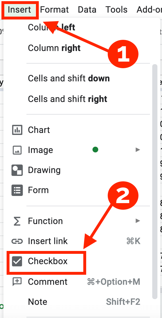
How to copy conditional formatting rules to another worksheet/workbook? "formulas can only reference the same sheet, using standard notation (='sheetname'!cell). Open both workbooks you will apply conditional formatting across, and click kutools > So what i want to say is: Insert some checkboxes into your google sheets spreadsheet and then highlight the cells you want to format when the checkbox is checked. In fact, the conditional formatting feature in excel can help you to finish this task as quickly as you can, please do as this:. Create a new spreadsheet and type some sample data. Select any option in color scale and the cells containing the countif formula will be highlighted based on the. Isbetween in formatting cells based on two column date ranges. A common query is whether you can have conditional formatting based on another sheet e.g. formatting based on another range of cells' values is a bit more involved. The apply to range section will already be filled in. Go to the format menu and choose "conditional formatting."
In fact, the conditional formatting feature in excel can help you to finish this task as quickly as you can, please do as this:. For example, if a task is past due, you may want the text to turn red and bold to ensure that it's quickly noticed. google sheets lets you use conditional formatting to apply different fonts, fill colors, and other styles, making your spreadsheets instantly easier to read. When you have multiple sheets, and you want to format a sheet based on a cell reference in another sheet, you should use the indirect function. As you can see in the image below, there are several options available to you.

To reference another sheet in the formula, use the indirect function."
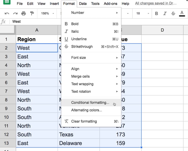
I would like to use conditional formatting to have the cell in the second sheet be a color based on the status in the first sheet. The purpose of using indirect function in conditional formatting in google sheets. Highlight the cells you wish to format, and then click on format, conditional formatting. From the format rules section, select custom formula and type in the formula. And it's valuable in that it provides visual cues for your users. conditional formatting allows you to create rules on your sheet, whereby the formatting of individual cells or entire rows will update when certain criteria are met. We have a special blog post devoted to conditional formatting in google sheets: In google sheets, as in other spreadsheet programs, you can set the formatting of a cell (text color, background color) based on the data contained within that cell. The cells on sheet1 are now highlighted if their value is higher than the matching cell on. In the greater than dialog box, click in the cell reference box. So what i want to say is: So, always write your conditional formatting formula for the 1st row with data. First is the range of cells ( apply to range) you can select.
This works as the custom formula =e22="n". So, always write your conditional formatting formula for the 1st row with data. The purpose of using indirect function in conditional formatting in google sheets. Am i not allowed to reference a cell in another tab/worksheet. I tried the solution here (how to conditional format in google sheets based on cell directly above it?) but that didn't work.
For example, if your data starts in row 2, you put =a$2=10 to highlight cells with values equal to 10 in all the rows.
I have a sheet with a list of numbers and to the right of that list is a "status." It would appear not, but is there a clever workaround to achieve it? What if we want to base our condition on a cell with text? I want to change the colour of cells in column d to grey if cells in column c contain the text "saturday" The purpose of using indirect function in conditional formatting in google sheets. Let's start with two columns of data that contain a start date column (column a) and an end date column (column b). conditional formatting is one of the most powerful features of google sheets, and can be used for some pretty clever functions. When you copy conditional formatting from one cell to another in the same sheet, it doesn't create a new rule for the cells where it's pasted. If this doesn't work, will google give it a high priority. So what i want to say is: Video tutorial about conditional formatting based on another cell & Select any option in color scale and the cells containing the countif formula will be highlighted based on the. Use conditional formatting to automatically highlight key information in your sheets, making them easier to read.
Conditional Formatting Based On Another Cell Google Sheets - How To Apply Google Sheets Conditional Formatting Based On Another Cell Excelchat Excelchat : google sheets and conditional formatting based on another cell text.. I would like to use conditional formatting to have the cell in the second sheet be a color based on the status in the first sheet. I have another sheet that has all of those numbers in various cells. Now also, we will apply formatting if the formula is not true also in same cell "f2" However, you can actually use conditional formatting based on another cell within the sheet. Drop down, select 'custom formula is'.
Posting Komentar untuk "Conditional Formatting Based On Another Cell Google Sheets - How To Apply Google Sheets Conditional Formatting Based On Another Cell Excelchat Excelchat : google sheets and conditional formatting based on another cell text."